The available features of the QuickControl depend on if the user has a license for the Basic or Advanced version. In the Basic version, Advanced features such as control of hardware devices and acquisition of 2D IR spectra will be present in “demo mode” - you can view the options but not use them.
There are three main sections of QuickControl - CONTROL mode, ACQUIRE mode and SETTINGS. There is also a built-in Calculator for calculating shaper parameters and a secondary program for controlling hardware called the Hardware Server.
Much of the shaper control is accomplished by controlling the arbitrary waveform generator (AWG) used to create the signals that drive the shaper. AWG is an abbreviation we will use often in this manual.
- Download and install the LabView 64-bit Runtime Engine.
- Download the QuickControl zip file and extract its contents to a directory anywhere on your computer. We’ll call that directory the “main directory”.
- Demo users can jump to Running QuickControl for the First Time.
- Install the LabView 32-bit Runtime Engine.
- Download the HardwareServer zip file and extract its contents to the main directory you created above.
- See the manuals for your specific PhaseTech instruments for listings of any additional required hardware drivers.
Demo:
- Run
PT_QuickControl.exein your main directory and choose the “Demo Mode” option when prompted for license information.
Basic and Advanced:
- Run
PT_HardWareServer.exein your main directory and ensure that all of the hardware settings are set to “OFF.” - Run
PT_QuickControl.exein the same directory and enter your Name and Serial Number when prompted for license information.
We recommend confirming normal operation of shaper or spectrometer hardware immediately before and after upgrading QuickControl or the HardwareServer.
- Download the zip file containing the updated version of QuickControl.
- Make a back up your current main directory.
- Extract the files in the QuickControl zip file (
PT_QuickControl_X.X.X.X.zip) into your main directory, overwriting any existing files with the same names. - If also upgrading HardwareServer:
- Extract the files in the HardwareServer zip file (
PT_HardwareServer_X.X.X.X.zip) into your main directory, overwriting any existing files with the same names. - Download the zip file containing the updated version of HardwareServer.
- Extract the files in the HardwareServer zip file (
- Run
PT_QuickControl.exe.
When upgrading QuickControl versions, all of your software settings should transfer. If any do not, QuickControl will show an error on the initial startup after upgrading and will generate a loaderrs file in the main directory. You can send this file to PhaseTech for support.
In addition to checking for errors on upgrade, we recommend confirming Visible Shaper Settings and QuickShape Calibration Parameters, both found under SETTINGS > SHAPER, before and after upgrade. Errors in Visible Shaper Settings can disable software safeguards against overdriving the visible shaper acousto-optic modulator (AOM) at 100 kHz, and can result in damage to the AOM crystal.
- Install
ni-labview-2020-runtime-engine_20.0.0_offline.iso - Install
ni-labview-2020-runtime-engine-x86_20.0.0_offline.iso - Follow the instructions for a normal upgrade.
To navigate to this screen, click the "CONTROL" tab at the top of the window.
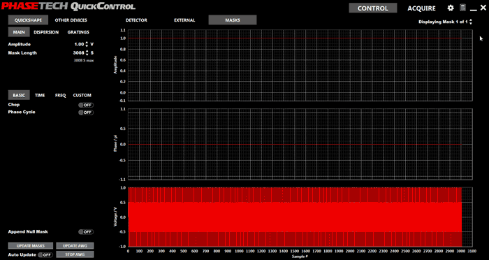
This section consists of two main parts - a Device Control column on the left-hand side of the screen with most of the screen taken up by the Control Display section. The Device Control column is used to control the pulse shaper (all QC Versions) as well as monochromators, delay stages, and shutters (QC Advanced). The Control Display will display data on the calculated pulse shaper mask and detector signals.
The right had side shows the calculated amplitude and phase masks as well as the RF waveform to be produced by the AWG. If multiple masks are to be output in sequence, you can change which mask is displayed by using the "Displaying Mask" control in the upper left.
The column on the left hand side is used to calculate waveforms and upload them to the AWG. At the top of this column are three tabs: "MAIN", "DISPERSION", and "GRATINGS".
The Main tab allows adjustment of the waveform amplitude and length.
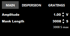
Power controls the maximum overall power of the RF waveforms. Possible values range from 0 (no output) to 100% (maximum output). At 100% a sine wave output, such as a basic mask, is at the maximum output level of the AWG. Adjusting the Power level will automatically set the corresponding Amplitude value.
Amplitude controls the maximum overall amplitude of the RF waveforms. Possible values range from 0 (no output) to 100% (maximum output). At 100% a sine wave output, such as a basic mask, is at the maximum output level of the AWG. Adjusting the Amplitude level will automatically set the corresponding Power value.
Older Version Note: Older versions of QuickControl may only have an Amplitude control. In these versions the possible values range from 0.0 (no output) to 1.0 (maximum output), with 0.0 and 1.0 corresponding, respectively, to 0% and 100% in newer versions.
Note: The PXDAC4800 AWG has built-in digital attenuation which reduces the amplitude of the output without decreasing the vertical resolution. If the PXDAC4800 is selected is used this feature is automatically used for amplitude values above ~0.27. Below this, the vertical resolution will be reduced to decrease the output amplitude. An external RF attenuator may be used to reduce the amplitude of the RF signal below 0.27 without losing vertical resolution. Contact PhaseTech for further details if needed.
Mask Length determines the length of each mask, in AWG samples.
For the AWG300, possible values range from 0 to 3008 in steps of 16. Each sample corresponds to 3.333 ns in the RF waveform.
For the PXDAC4800, running at 1200 MHz sampling rate, the possible values range from 0 to 12000. Each sample corresponds to 0.83 ns in the RF waveform.
The Dispersion tab allows control of GVD and TOD correction:
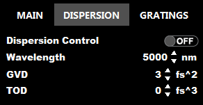
Dispersion Control determines whether dispersion control is applied to the masks output from the AWG. If Dispersion Control is set to "On", then the Wavelength, GVD, and TOD parameters are used to calculate the dispersion control phase mask. If Dispersion Control is set to "Off", then the Wavelength, GVD, and TOD parameters have no effect on the output waveform.
Wavelength should be set to the center wavelength of the mid-IR pulse. If the center wavelength of the mid-IR pulse changes significantly, the dispersion parameters may need to be redetermined.
GVD determines the amplitude of the quadratic dispersion term applied to the shaped pulse.
TOD determines the amplitude of the cubic dispersion term applied to the shaped pulse.
The Grating tab allows control of the motorized rotation stages.
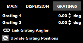
Wavelength and Frequency can be move the incident grating to approximately the correct angle for a given wavelength or frequency, this is a beta feature. Adjusting either Wavelength or Frequency will adjust the other appropriately. They will also automatically update when the angle of the incident grating is adjusted. Which grating is considered the incident grating is set in the Settings, as described below. The abbreviation "wn" stands for wavenumbers.
Grating 1 and Grating 2 can be used to rotate the gratings to the desired angle.
If Link Grating Angles is turned on, then when one of the gratings is rotated by a certain number of degrees, the other grating is rotated by an equal amount in the opposite direction. This feature is useful for tuning the center wavelength of the shaper.
Update Grating Positions can be used to read the current positions of the gratings. This can be useful if the grating positions have been changed using the microcontrollers.
Underneath these first set of options, there are four tabs: "BASIC", "TIME", "FREQ" AND "CUSTOM".
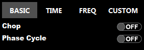
The option simply outputs a basic mask which will generate a basic shaped pulse. (Dispersion control will be applied if selected in the global parameters.)
The Chop option will generate a mask sequence two masks long where the first mask is a basic mask and the second mask is a zero amplitude mask (in other words, no mask).
This tab is used for time-domain experiments and scans.
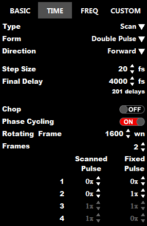
Form determines if the shaper outputs a single pulse or a double pulse. A double pulse consists of two equal amplitude pulse, one that is scanned in time and one that is fixed in time. Possible values are "Double Pulse" and "Single Pulse".
Direction determines the direction (in time) that the pulses are scanned, relative to a basic pulse or the fixed pulse. Possible values are "Backward" and "Forward". "Backward" means that the scanned pulse arrives before the fixed pulse and "Forward" means that the scanned pulse arrives after the fixed pulse. (For 2D IR measurements, the "Backward" option should generally be used.)
Type determines if a scan of multiple delays will be used or if a single fixed delay will be used. Possible values are "Scan" and "Single". If "Single" is chosen, the single delay value will be equal to the value of the Final Delay parameter. If "Scan" is chosen, the scan will begin at a delay value of 0 fs, and continue in steps determined by Step Size, with the final delay set by Final Delay.
Chop turns on chopping of the scanned pulse. In this case, each time delay is used for 2 sequential laser shots, the first without the scanned pulse and the second with the scanned pulse.
Phase Cycling turns on phase cycling. In this case, each time delay is used for up to 4 sequential laser shots. For each shot the scanned and fixed pulse can have different phases as determined by the phase table, as described below.

NOTE: Turning on the Chop option will turn off the Phase Cycling option and vice versa. Frames determines the number of frames in the phase cycling scheme. The number of frames is the number of consecutive pulses used at each time delay.
The phase table (shown below) determines the phase of pulses for each frame of the phase cycling scheme. The number of enabled rows is determined by the value of Frames. Which columns are enabled is determined by the value of Form.
The left-most column of numbers are labels indicating the frame number. The Scanned Pulse column determines the phase of the scanned pulse in each frame. The Fixed Pulse column determines the phase of the fixed pulse in each frame. To change each phase value, either use the arrows next to each phase or enter a number between 0 and 2 into the boxes.
Rotating Frame determines the rotating frame used for the scanned pulse. To turn off, set to 0. Otherwise a ωrfτ term will be added to the phase of the scanned pulse, where ωrf is the value of Rotating Frame (converted to 1/fs) and τ is the delay.
This tab is used for frequency-domain experiments and scans.
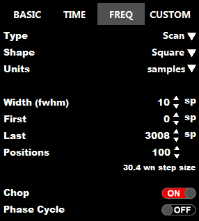
Units determines the units used for the other parameters in the tab. Possible values are "samples", "nanometers", "wavenumbers" and "THz". If the value of Units is changed, the values of the affected parameters will automatically be converted to the new units. In cases, were the conversion factor varies across the mask length, the conversion factor at the center of the mask is used.
Shape determines the shape of the pulse in the frequency domain experiment. Possible values are "Square", "Gaussian", "Lorenztian", "Etalon", and "Reverse Etalon". Note that the "Etalon" and "Reverse Etalon" options are only compatible with units of "wavenumbers".
Type determines if a scan of multiple frequencies will be used or if a single fixed frequency will be used. Possible values are "Scan" and "Single". If "Single" is chosen, the single delay value will be equal to the value of the First or Last parameters depending on the value of Units.
First determines the center position for the first mask in a scan, in the specified units.
Last determines the center position for the last mask in a scan, in the specified units.
Steps determines the total number of steps performs in the scan.
Chop turns on chopping of the scanned pulse. In this case, each frequency is used for 2 sequential laser shots, the first without the scanned pulse and the second with the scanned pulse.
This tab allows users to upload their own custom mask sequences.

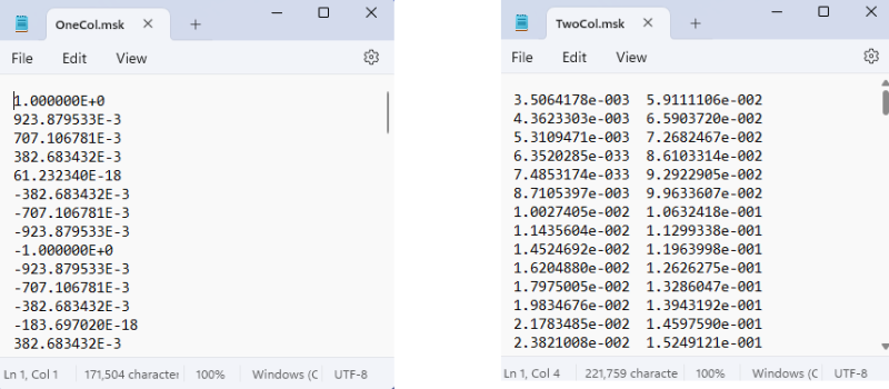
Each mask in the sequence should consist of a tab-delimited ASCII text file with a ".msk" extension.
The .msk file can either contain one or two columns. If the file contains only a single column, that column represents relative RF voltage values (values between -1 and 1). If the file contains two columns, the first column represents amplitude values (values between 0 and 1) and the second columns represents phase values (values between 0 and 2p—values outside this range will wrap back in). Each row in the file corresponds to a sample in the mask.
The Amplitude/Power settings ("MAIN") scale the amplitude of a custom mask.
Dispersion Control and Bragg Correction settings ("ADVANCED") apply to two-column (amplitude / phase) custom mask files, but not to one-column (RF) custom mask files.
A mask sequence is specified by placing multiple mask files in the same folder. The order is determined by alphanumeric sorting of the file names.
Mask Directory specifies the location of the mask files. The folder path may be entered manually, or you can click the BROWSE DIRECTORY button to specify the location. Once the location is entered, you can click the OPEN DIRECTORY button to view the contents of the directory.Mask Order will display any masks found in the mask directory. The order of the filenames in this display is the same order that the masks will be output from the AWG. To change the order, modify the filenames and then click the REFRESH LIST button.
Calculated masks can be saved externally. Right clicking on the bottom graph in the MASKS tab (Voltage / V) gives is a "Save Masks" option. Selecting this option deletes any masks currently saved in the "\masks" subfolder of the QuickControl directory and replaces them with the currently calculated masks (one file per mask).
Each mask is saved as a single column of values, with each value corresponding to the relative voltage output of the AWG card (values ranging between -1 and 1). Relative voltage values start at Sample # 0 (row 0) and continue in order.
This section is used to control one or two monochromators. If two monochromators are installed, use the PRIMARY/SECONDARY tabs to select the controls for the desired monochromator. If only one monochromator is installed, the PRIMARY/SECONDARY tabs are disabled and only the controls for the primary monochromator will be displayed.
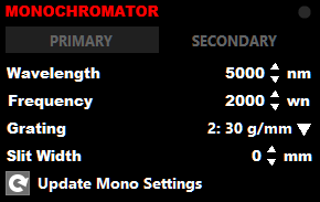
The Wavelength and Frequency controls set the center wavelength or frequency of the monochromator. Entering a value into the Wavelength control will automatically update the Frequency control with the corresponding frequency and vice-versa.
The Grating control will move the monochromator to the selected grating, if the monochromator has a motorized grating turret.
The Slit Width control will set the entrance slit width on the monochromator, if the monochromator has a motorized entrance slit.
The Update Mono Settings button will read the current central wavelength, grating and slit width of the monochromator and updated the displayed values in QC. Use if another program is used to change these values or they otherwise differ from the displayed values.
This is one of two delay stage controls. In 2DQuick products this stage is the one inside the 2DQuick enclosure which sets the delay between the shaped pulse and the probe pulse. This can also control any delay stage through the use of the plugin system.
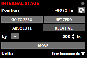
To the right of the "Internal Stage" label is a movement indicator which will turn red with the stage is currently in motion.
Position displays the current position stage. Click the refresh button to the right of the display to update the displayed value if the stage position is moved outside of QC.
The Go To Zero button moves the stage to zero delay.
The Set Zero button sets to current stage position (as displayed in the Position indicator) to be zero delay.
The Motion Type selector determines whether motion commands are made in relative to the zero position ("Absolute") or relative to the current position ("Relative").
The Motion Sign button negates the sign of the motion commands. The button label changes from a "+" sign to a "-" sign when the command is being negated. This makes it easy to move the stage back and forth by a fixed amount, for example, when aligning the delay stage.
The controls for the External Stage are identical to the those for the Internal Stage.
The shutter control consists of a single option, to switch the stage of the shutter from open to closed or vice versa.
Control Display has four display sections: Detector, Image, External and Masks.
Three controls are shared by the Detector, Image, and External display sections. These controls control the acquisition of data. Also when a data is acquired the graphs in all three sections are updated, even if they are not currently being displayed.
The first control, Average, determine the number of laser shots that data will be collected for during each acquisition. Certain circumstances may required a specific multiple of laser shots to be collected, such as 2 or 4 shots, for proper processing and display of data.
The second shared control is the button to begin an acquisition. The third control is the continuous acquisition option, symbolized by infinity symbol. The behavior of the Begin Acquisition, and the data acquisition, depends on if the continuous acquisition options is enabled or disabled.
If the continuous acquisition option is off, then only a single acquisition will be carried out. However, if continuous acquisition is on, each acquisition will be immediately followed by another acquisition in an infinite loop until one of three events occurs: (1) When acquisition begins the Begin Acquisition button changes to a Stop Acquisition button. Clicking this button will stop the acquisition loop after the current iteration and turn off continuous acquisition. (2) Turning off the continuous acquisition option will also stop the acquisition loop after the current iteration. (3) If an error code is produced during acquisition, the continuous acquisition options will be turned off.
This display section is for viewing signal on a detector, if a detector is setup for use with QuickControl. QuickControl has built-in support for a number of detectors but unsupported detectors may also be used through a detector plugin. The section consists of two graphs as well as a few controls.
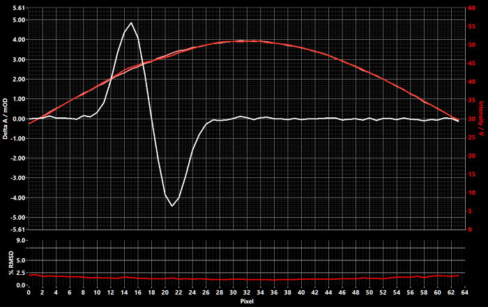
The two graphs share the same x-axis. The x-axis is the pixel columns of the detector from 0 to N-1, where N is the number of pixel columns that the detector has. The x-axis can also be calibrated to show frequency or wavelength at each pixel column as described below. Changing the limits of the x-axis changes the limits for both graphs.
The top graph shows displays multiple types of data on two different y-axes. The first type of data shown is a difference spectrum, or pump-probe spectrum. This is calculated as the negative logarithm of the ratio of consecutive pairs of laser shots. The value is then averaged over the number of laser shot pairs collected. The pump-probe spectrum is displayed as a white trace and on the left y-axis. The values of the left axis are Delta OD (ΔOD) in units of mOD (10-3 OD).
Note: In order for the pump-probe spectrum to be calculated properly, data must be collected for an even number of laser shots.
The second type of data shown is an intensity spectrum. There are two intensity traces, one shown in red and the other in pink. The two traces differentiate between two types of intensity data depends on the options selected, as described in more detail below. The intensity traces are displayed on the right y-axis. The values of the left axis are intensity in units proportional to Volts, although no absolute voltage calibration or linearity is assumed.
The y-axis each had a number of scaling modes affecting how the axis limits (minimum and maximum values) are updated when new data is displayed:
- AutoScale In this scaling mode, the axis limits are automatically increased or decreased to match the range of the values in the data.
- Smart AutoScale In this scaling mode, the axis limits will automatically increase if the range of values in new data exceeds the current axis limits. However, if the data range decreases, the axis limits will not change.
- AutoScale Once Selecting this scaling option will scale the axis one time based on the next collected data. No further scaling will be done until another option is selected.
- Keep Symmetric When this option is enabled, the range of the y-axis will be kept symmetric about zero. That is, the negative axis limit will be set equal to the maximum axis limit. This option is only available for the Delta OD axis.
To the upper right of the detector graphs is a dropdown menu with a number of options controlling how the data is displayed. The menu has a number of sections,
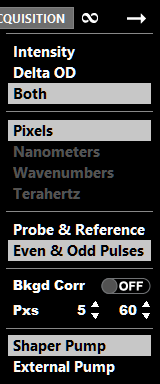
The first section sets which traces are displayed in the upper graph. There are three options corresponding to (1) display only Intensity traces (Delta OD trace hidden), (2) display only the Delta OD trace (Intensity traces hidden), (3) Both show both types of traces.
The second section determines the units used for the x-axis of both graphs. The first option, Pixels, uses pixel numbers - 0, 1, 2, ... - for each pixel column in the detector. The other three options allow the display of data as function of frequency or wavelength in nanometers, wavenumbers, or terahertz. These three options will be disabled unless a detector calibration method is selected in the Detector settings. WARNING The user is responsible for the accuracy of this calibration. No level of accuracy is presumed.
The third section determines the types of intensity data displayed as the red and pink intensity traces. The first option, Probe & Reference displays the average signal from probe region on the red trace and the average signal from the reference region on the pink trace. The second option, Even & Odd, displays data from the probe region only. In this case, the red traces show the intensity signal averaged over even laser shots only and the pink traces show the intensity signal averaged over odd laser shots only.
The fourth section allows the application of a linear background correction to the Delta OD data. When enabled, the linear background correction is performed using the two pixels specified. The x-y values at these two pixels are used to define a line and this line is extrapolated to all pixel columns and subtracted from the signal. The pixel columns set here are also used for the linear background correction option in Acquire mode.
The fifth and final section determines which chopper signals is used to correct the phase of the Delta OD signal from acquisition to acquisition. The first option, Shaper Pump, should be selected when the shaper output is being used as the pump pulse and is being chopped. The second option, External Pump, should be selected when an secondary excitation pulse is used, such as a UV/visible actinic pulse. Note: For these options to function properly, the proper chopper signals must be provided as external channels and the index of the respective channels specified in the Detection settings.
This section is only enabled if the detector has more than two rows of pixels. The section consists of two displays and a number of controls.

The main display is an intensity plot showing the average intensity on each pixel of the detector. The color range is automatically scaled to entire range of values in each image. The display includes two overlay features - a cursor and region of interest highlight boxes. Both overlays can be turned on and off with the controls to the right of the display.
The secondary graph displays 1D data sets derived from the image in different ways. The type of 1D data set display is determined by the selection of the dropdown box to the upper right of the graph. There are a number of options:
- Cursor Row displays a slice through the image data at the pixel row specified by the current location of the cursor
- Cursor Column displays a slice through the image data at the pixel column specified by the current location of the cursor
- Probe Region displays a vertical average of the image data over the rows specified by the probe region of interest
- Reference Region displays a vertical average of the image data over the rows specified by the reference region of interest
- Row Average displays a vertical average over all rows of the image data
- Column Average displays a horizontal average over all columns of the image data
Directly beneath the secondary graph is the controls for the cursors. The cursor display can be turned on and off. Note that the cursor position can still be used for displaying specifying rows and columns to display in the secondary graph when the cursor display is off.
The Row and Column position of the cursor can be specified with the corresponding controls. The Value of the image data at the cursor position is also displayed. When the cursor display is on it can be moved by dragging the cursor with the mouse. The Row, Column, and Value control values will updated with the new position when the cursor is dragged in this manner.
The next set of controls determine the regions of interests (ROI) used in data acquisition and processing. The regions of interest specify which pixel rows contain different types of signals.
First, it is possible to turn on and off the display of highlight boxes on the main image graph. These boxes provide an visual indication of the pixel rows selected for each region. Turning the display on and off does not affect the use of the ROIs through QuickControl, simply the display of the highlight boxes.
Below, is a list of the available ROIs and their defining parameters. Each ROI is specified by a Center Row and a Height. As these values are changed the ROI highlight boxes, if on, will update to show the selected rows on the image plot.
Finally, the Save Image Data will save the current image data to a text file. Clicking the button will open a dialog box for specifying the file location.
These graphs display signals that might be acquired simultaneously with the signals from the detector but are external to the detector itself. That is, signals not from the pixels of the detector. Examples include the detection of the voltage on the synchronization channel of the AWG in a PhaseTech pulse shaper, or the signal from an optical chopper, but could be any external signal.
The presence of external signals requires that the detection hardware be present and setup to detect external signals and that the number of external signal channels be set to a number greater than zero in QuickControl settings.
The are two graphs present in this section. The top graph shows the average signal on each external signal channel over the number of last shots acquired. The bottom graph shows a plot for each external channel, showing the signal for every laser shot acquire. To the right of the graph there is a legend showing the plot color for each external channel plot. This legend can also be used to the turn the display of each plot on or off.
These graphs display various components of the most recently calculated sequence of masks. From top to bottom, there are graphs for the amplitude component of the masks, the phase component of the masks, and the resulting RF signal.
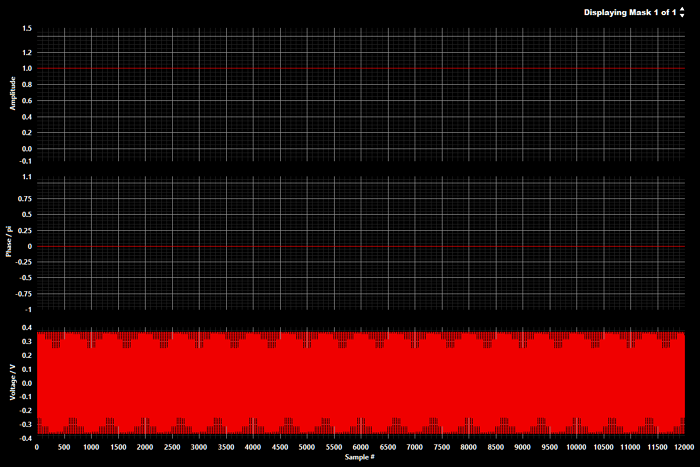
In the upper right-hand corner of this section is a control which shows the number of masks in the most recently calculated mask sequence as well as the mask number for the mask currently displayed in the graphs. Change the value of this control to change which mask is displayed.
The top graph displays the value of the amplitude mask at each sample position. Values are in normalized amplitude and range from 0 to 1.
The middle graph displays the value of the phase mask at each sample position. Values are in units of π radians and are wrapped into the range of -1 to +1. (For example, 1.5π is wrapped to -0.5π.)
The bottom graphs displays the RF signal output from the AWG at each sample position. Values are proportional to Volts. The signal should be observed when the output of the AWG is sent to an oscilloscope.
The three graphs share a common x-axis in units of AWG samples. Adjusting the range for the single x-axis applies to all three graphs.
Acquire mode is used for collecting various types of data and consists of four sections:
- 1D & 2D - for collecting 2D spectra and 1D pump-probe spectra
- MONO SCAN - for collecting intensity spectra by scanning the central wavelength of the monochromator
- GVD SCAN - scans the GVD and/or TOD applied by the pulse shaper and measures a corresponding signal, such as SHG intensity
- CUSTOM - conduct custom pulse shaping experiments via a user-written plugin
The control bar at the bottom of the Acquire mode window is common to all four sections.
The control bar is used to start, stop and pause experiments, sets the filename for experiments, sets a comment line that is saved with the experiment data and displays the current progress during a scan.
At the left-most side of the control bar are a set of four buttons which control the run state of the experiment. From left to right the buttons are Start, Single, Pause, and Stop. At first startup or whenever an experiment is not running, only the Start and Single button are enabled. The Pause and Stop buttons are disabled unless an experiment is in progress.
The Start button will start an experiment with all the current setting. The experiment will continue collecting scans until the the final scan is reached or exceeded.
The Single button will also start an experiment but will also stop the experiment after a single scan. It does this by setting the final scan parameter (see below) to "1". So this button is simply a shortcut for manually changing the final scan parameter to 1 and clicking the Start button. It is also possible to increase the number of scans during the single scan if you change your mind and want to continue scanning.
The Pause button will pause the experiment until the button is clicked again. The icon for this button will change to have a red background when the experiment is paused. There may be a small delay before the experiment pauses if the button is clicked in the middle of a step.
The Stop button can be used to stop an experiment before it reaches the final scan. Once clicked you will be presented with three further options to confirm stopping of the experiment. This prevents accidental stopping of the experiment and loss of data. The experiment continues to collect data until an option is selected. The first option is to Cancel the stopping of experiment. If Cancel selected the experiment continues as if the Stop button was never clicked. Another option is Stop Now which will stop the experiment as soon as possible in the middle of the current scan. If selected, this data from the current scan may be inaccurate or incomplete. The final option is After Current Scan, which stops the experiment after the currently running scan completes. This preserves the data of the current scan. This option stops the experiment by changing the final scan parameter to equal the current scan number. So is also possible to increase the number of scans during the scan if you change your mind and want to continue scanning.
Note: If an experiment is started, QC will check to see if there is existing data with the same filename. If there is a warning will be displayed and you will get an option to either overwrite the existing data or cancel the experiment so that you can choose a different file name.
The next section of the Control bar, are the filename controls, which determine the filename that will used for saving the various files the experiment generates.
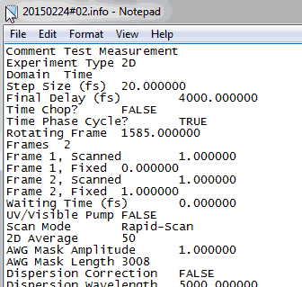
The File Prefix control sets a text string that will be used at the beginning of all files generated by the experiment. This is automatically set to the a string based on the date that QC was opened in the format "YYYYMMDD" followed by a "#" as a separator. However, this string can be changed by the user as desired.
Directly to the right of the File Prefix control is the Experiment Number control. This is a zero-padded two-digit number which gets appended to the File Prefix for any files generated by the experiment.
The Auto-Increment when enabled, will automatically increment the Experiment Number by one at the end of each experiment.
Click More File Options... to quickly go to the QC Settings section that provides more options for managing the saving of experiment files.
The Comments control is simply a large text box for adding user comments or notes to the info file which is saved with each experiment. It has not effect on the experiment.
The right-most section of the Control Bar is used to display the progress of the experiment as well as to set the end point of the experiment.
This is the most commonly used section of Acquire mode. Use this section of collect 2D spectra (2D IR or 2D visible) as well as collect pump-probe (1D) spectral kinetics.
This section consists of two subsections: Setup and Graphs.
The Setup sub-section is used to set all the necessary experimental parameters for a 1D or 2D experiment. There are two different ways to set the parameters for an experiment. The first is through the use of experiment presets and the second is to manually set each parameter.

The Experiment Presets column begins with a list of available presets, sorted alphabetically. If there are a large number of available presets, you may need to scroll the list to see them all.
Below the preset list there are three buttons:
- Load Selected Preset, Loads the parameters stored in the currently selected experiment present.
- Delete Selected Preset, Deletes the currently selected experiment preset.
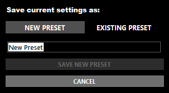
Save Current Settings as a Preset, Saves the currently chosen experimental parameters as a preset. Once clicked, the preset display will change to present a few options about how to save the new preset:
-
New Preset - Create a new preset with a name as entered in the provided input.
-
Existing Preset - Choose from the provided list of existing presets to overwrite the preset parameters with the current parameters.
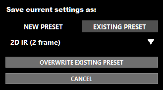
- Cancel - Cancels saving of the preset and returns to the standard preset display.
-
New Preset - Create a new preset with a name as entered in the provided input.
NOTE: If factory-default experiment presets are modified or deleted, they can be restored using the "Restore Experimental Presets" button in the Settings. See the Settings section of the manual for more details.
NOTE: Each preset is saved as a text file in the "presets" subfolder of the main QuickControl directory. If desired, presets can be created, deleted or modified using these text files directly. QuickControl may need to be restarted before any changes made to the text files are in effect.
The Experiment Parameters column allows the user to control the different parameters that control how a particular experiment is carried out. Any displayed parameter can be set in any order. However, there is a certain logical flow to selecting options from the top down. The first selection to make is whether to conduct a 1D Experiment or 2D Experiment.
A 1D Experiment is a traditional pump-probe, transient absorption experiment where the delay between the pump and probe pulses is scanned using a translation stage and a transient absorption spectrum is measured at each delay. Typically the spectrum at each delay is measured by averaging over 100s or 1000s of laser shots. Additionally, a number of scans of the the delays are typically measured and averaged together.

There are two types of 1D pump-probe scans that can be run: a mid-IR pump, mid-IR probe 1D experiment and, if an external delay stage is equipped, a UV/visible pump, mid-IR probe 1D experiment. The options for the two types of scans are the same, except that the delays for mid-IR pump experiments are specified in femtoseconds while the delays for UV/visible pump experiments are specified in picoseconds.
The main parameter to set for 1D pump-probe experiments is the values of the pump-probe delay that will be scanned over during the experiment. There are three different ways to set these delays: Exponential, Linear, and List.
When using exponential delays the step size from one delay to the next increases exponentially with the value of the delay. This allows you to collect data with closely spaces delay points near zero where fast dynamics may be taking place and also spend less time measuring data at longer delays where less delay points are needed.
The first step in setting up an set of exponential delays is to choose a target First and Last delay for the scan. (The first delay is often negative.) Due to the math involved in calculating the exponential delays, it is generally not possible to hit the target delays exactly. Therefore, QC will display the actual first and last delays that result from the calculation of the exponential delays. It is then possible to increase or decrease the target first and last delays, as desired, until you are satisfied with the actual first and last delays.
The Minimum Step Size sets the delay step size (in either direction) when at zero delays. The delay steps then increase from this number with increasing delay.
The Weighting Factor determine how quickly the delay steps increase with increasing delay. The higher the value, the faster the delay step increases and the smaller number of steps will take place within a given delay range.
The simplest delay scheme, delays are scanned with a fixed step size from the first delay to the last. First specifies the starting delay for the scan. Last specifies the final delay for the scan. Step Size specifies the size of steps to make between the First and Last delays.
Note: The value of First and Last must be an integer multiple of the Step Size. QC will enforce this condition automatically.
This delay mode allows you to specify an set of arbitrary delays to scan. Delays are specified as a list of comma separated values. For example:
-50, -10, -8, -6, -4, -3, -2, -1, 0, 1, 2, 3, 4, 6, 8, 10, 50, 100, 200, 250, 300, 350
The current list can also be saved to a text file using the Save to File button or a existing file can be loaded into the list using the Load from File button.For all three delay modes, beneath the delay selection section is an indicator which displays the total number of delays. This display updates whenever a change in the delay settings is made.
Additionally, there is an option to reduce the number of negative delays used in Exponential or Linear Delay modes. This feature is not available for List mode. In 1D pump-probe experiment it is generally useful to collect data at a number of negative delays. This provide a good background signal for comparison with the pump-probe signal at positive delay. However, in doing so, you can spend a large amount of the total experimental time collecting data where there is not signal.
For example, if you scan positive delays out to 1000 ps, you might want to scan negative delays out to -100 ps. Using Exponential delays, with a Minimum Step Size of 0.016 ps and a weighting factor of 0.18 would result in a set of 99 delays. Of these 99 delays, 42 would be at negative time delay! Almost half the experimental collection time would be spent at delays with no signal.
The Reduce Negative Delays option can be enabled to improve this. The Keep every and When less than parameters specify how to reduce the negative delays - which negative delays to get rid of. The feature keeps all delays that are smaller (less negative) than the When less than parameter and then, starting with the first delay larger than this parameter, keeps every 2nd, 3rd, 4th,... delay thereafter.
Continuing with the above example of scanning from -100 ps to 1000 ps. The 42 negative delays are:
-92.78, -78.62, -66.61, -56.44, -47.81, -40.51, -34.31, -29.07, -24.62, -20.85, -17.66, -14.95, -12.66, -10.71, -9.064, -7.668, -6.484, -5.482, -4.632, -3.912, -3.302, -2.784, -2.346, -1.975, -1.66, -1.393, -1.167, -0.9754, -0.8131, -0.6755, -0.5589, -0.4601, -0.3763, -0.3054, -0.2452, -0.1943, -0.1511, -0.1145, -0.08345, -0.05716, -0.03488, -0.016 ps
If the instrument response function of our experiment was say, 250 fs, we might want to keep negative delays smaller than -500 fs, in order to make sure we did not cut off the rise of the pump-probe signal. Therefore we would set the When less than parameter to -0.5 ps. If we set the Keep every parameter to "2nd" the number of negative delays would be reduced to :
-78.62, -56.44, -40.51, -29.07, -20.85, -14.95, -10.71, -7.668, -5.482, -3.912, -2.784, -1.975, -1.393, -0.9754, -0.6755, -0.4601, -0.3763, -0.3054, -0.2452, -0.1943, -0.1511, -0.1145, -0.08345, -0.05716, -0.03488, -0.016 ps
The number of negative delays is now 26, almost a 50% reduction while still providing data over a useful range of negative delays.
After the delays settings, the Shots to Average parameters specifies the number of laser shots over which to average the signal at each delay step.
Finally, it is possible to turn on a linear background correction, applied to the average pump-probe spectrum at each delay. The two pixel columns used for the background correction are specified in CONTROL mode.
A 2D experiment measures a pump-probe as a function of the excitation frequency. The excitation frequency dependence can be measured in either the time-domain or the frequency-domain.
When measured in the frequency-domain, the spectrum of the pump pulse is narrowed to some fraction of its overall bandwidth and a pump-probe spectrum measured. The pump-probe spectrum is then measured for a series of narrowed pump pulses with different center frequencies (within the bandwidth of the original broadband pump pulse). The pump-probe spectrum for each excitation frequency is then directly plotted as a function of excitation in a 2D plot.
When measured in the time-domain, the pump pulse is split into two pump pulses and the pump-probe spectrum is measured as a function of the delay between the two pump pulses. The collected data is then Fourier transformed over delay axis in order to plot the signals as a function of excitation frequency.
PhaseTech pulse shapers and 2D spectrometers are capable of operating in both time-domain and frequency-domain mode. However, time-domain measurement is most commonly used because it measures the 2D spectrum with higher time-resolution than the frequency-domain approach. 2D spectra measured in the time-domain thus have more accurate information about the dynamics of the system than spectra measured in the frequency domain.
The first parameter to set when setting up a 2D experiment is whether to measure the spectrum in the TIME DOMAIN or the FREQ DOMAIN. Once selected the relevant parameters for each time of experiment will be displayed. These controls match those in CONTROL mode for time and frequency domain shaping, so refer to those sections of the manual for details.
Following the specification of the main time- or frequency-domain scanning parameters there is optional section of two parameters related to the use of an UV/visible actinic pulse for a Transient 2D measurement. The first parameter turns on or off the use of this actinic pulse while the second parameters sets the delay of this pulse. These parameters will be disabled if the External Stage hardware option is disabled in the Hardware Server.
Experiments can be collected in one of two different acquisition modes: Rapid-Scan acquisition or Step-Scan acquisition. During an experiment, a series of different shaper masks (a mask sequence) must be applied and the corresponding detector signal measured. Typical the signal for each mask must be measured many times and the averaged in order to achieve good signal-to-noise. The two acquisition modes differ in the way the mask sequence is scanned and the signals are averaged.
Step-Scan acquisition works by repeatedly applying the same mask to the shaper and averaging the detector signal for multiple laser shots before switching the applied mask to the next one in the mask sequence. After scanning through all the masks in the sequence, and averaging at each point, the detector signals are processed into a 2D spectrum. The processes is then repeated as necessary, averaging successive spectra together until the desired signal-to-noise is achieved.
On the other hand, Rapid-Scan acquisition, applies a new mask in the mask sequence on a shot-by-shot basis. The detector signal for each mask is similarly collected on a shot-by-shot basis and the signals can be processed into a 2D spectrum using the minimum number of laser shots possible. These "minimum shot" spectra can then be averaged as desired until good signal-to-noise is achieved.
Because Rapid-Scan mode modulates and collects the signal at higher rates it provides a signal-to-noise advantage over Step-Scan mode. Additionally, it minimizes the number of laser shots (and thus time) required to achieve a desired signal-to-noise whereas Step-Scan mode requires the user to chose the number of pulses to average starting the experiment. It is highly recommended to use Rapid-Scan mode whenever possible. The primary reason to use Step-Scan mode is if the shaper is being used with a detector that is not able to collect signals on a shot-by-shot basis.
Each of the two acquisition modes requires setting a parameter to control how the data is averaged.
For Rapid-Scan mode, the parameter specifies the number of 2D spectra to be averaged in memory before saving that averaged spectrum to a file. Multiple files of averaged spectra will be saved until an experiment is stopped.
For Step-Scan mode, the parameter sets the number of laser shots to be averaged at each mask in the mask sequence.
Additionally, for Rapid-Scan mode, the shaper masks should be setup in advance of starting the experiment. Click the Setup Shaper button before starting the experiment if any changes have been made to the mask sequence. For example, changing the Waiting Time Delay does not affect the mask sequence, so if the shaper has previously been setup before making changes to Waiting Time Delay, it would not need to be setup again. However, changes to the Time- or Frequency-domain scanning parameters would required clicking the Setup Shaper button to apply those changes.
It is also possible to turn on the use of custom masks when conducting a 2D experiment. In do so properly, a series of steps must be taken:
- Turn on the Use custom masks option at the bottom of the list Experimental Parameters.
- Set the experimental parameters in Acquire mode to best match those of your customers - scanning the same number of delays/frequencies, chopping or phase cycling, the number of frames, etc.
- In Control mode, upload the series of Custom masks to be used in the experiment.
- Do NOT click the "Setup Shaper" button before beginning the experiment.
The waiting time delay is the delay between the pump and probe pulses in a frequency-domain 2D experiment or the delay between the second pump pulse and the probe pulse in a time-domain 2D experiment. The controls for specifying waiting time delays are the same as for specifying delays in 1D experiments. Please review those sections for more detail before continuing.
If a single waiting time delay is specified, the waiting time will be constant through the experiment. The simplest way to specify a single waiting time delay is select LIST mode and enter just a single value.
If a series of waiting times are specified, then 2D spectra are measured at each waiting time delay in sequence. The number of scans collected, specified in the Acquire mode Control Bar, at each waiting time delay is the same for each delay. For example, if the number of scans is set to 10 and the number of waiting time delays specified is 5, then 50 total scans will be collected before the experiment ends.
One consquence of this is that the spectra measured at each waiting time delay will be collected with the same amount of averaging. Since signal amplitudes are large waiting time delays are typically smaller than signal amplitudes at short waiting time delays, it may be desirable to perform more averaging spectra at large waiting time delays. To do so, use the LIST mode of setting the waiting time delays and list larger waiting times multiple times. For example: 0, 50, 100, 100, 200, 200, 200, ... In post-processing spectra acquired at the same waiting time delay can then be further averaged together for better signal-to-noise.
Depending on the native signal-to-noise of an experiment as well as the spectral profile of the signal, background correction techniques can often be used to grealty in prove the signal-to-noise of an experiment. Many user chose to perform the background correction during post-processing. Doing the background correction in post-processing allows for the effect of the background correction on the data to be evaluated as well as the comparison of different background correction approaches.
However, it can also be done on-the-fly during the collection of spectra by turning on the Apply Background Correction option. This option applies to both 1D or 2D experiments. When enabled, the pixels specifed for background correction in Control mode are also used in Acquire mode.
Activate the Settings screen by clicking the gear icon at the top right of the screen. There are four sections of settings: General, Shaper, Detection, and Other Devices.
There are also two buttons, "SAVE ALL VALUES" and "LOAD ALL VALUES", which are visible from each of the four Settings sections. These buttons save and load all the options and data values in the QuickControl software. The values are automatically saved when QuickControl is closed and loaded each time the software starts up. You can also manually save or load the values but using the Ctrl+S and Ctrl+L key combinations from anywhere in the software.
This section contains general settings and information for QuickControl and settings unrelated to control of the shaper, detector or other hardware devices.

These setting affect the destination of the files generated and saved during Acquire mode experiments.
The Main Data Directory specifies the primary location in which files will be saved. All automatically saved experiment files will be saved somewhere within this directory. The Backup Directory specifies a second location (perhaps a network location or external drive) where a second copy of all automatically saved experiment files are saved. The location of these directories can be specified by entering the full path of the directory in to the box or by browsing for a directly using a dialog box. To browse for a directory, click the "browse" button. The use of the backup directory can be turned on or off using the ON/OFF switch directly to the right of the "Backup Directory" label.
The other options determine is subfolders are used with the main directory (or backup directory) to further organize the experiment files. There are two subfolder options:
Experiment Subfolder when on, saves experiment files in a subfolder based on the type of experiment being conducted in Acquire mode. 1D & 2D experiment files are saved to a "MAIN" subfolder, MONO SCAN files are saved to a "MONO" subfolder, GVD SCAN to "GVD", and CUSTOM to "CUSTOM".
Date Subfolder additionally saves experiment files into a subfolder based on the date. There are a number of options:
- Year - subfolder name is set to the four-digit year, such as "2017"
- Month - subfolder name is set to the four-digit year followed by the two-digit month, such as "201704"
- Day - subfolder name is set to the four-digit year followed by the two-digit month followed by the two-digit day, such as "20170423"
- Each - subfolder name is set to full Filename Prefix as specified in the Acquire mode control bar, such as "20170423#1". This option will save the files for each experiment to their own subfolder.
Record Initial Spectrum applies to 1D & 2D experiments. When each experiment starts, the average intensity on the detector will be averaged over 100 laser shots and then saved to a file. This provides a snapshot of the probe pulse spectrum at the start of the experiment which can be used for spectral calibration or other purposes.
The Restore Factory Experiment Presets will restore the set of standard presets for 1D & 2D experiments. If the current list of presets contains new presets that are not a part of the factory set, these new presets will be retained even after the restoration. However, any change you have made to the standard presets will be overwritten and lost. If you like you can make a copy of the presets before restoring the presets.
License Name shows the name associated with the license currently in use. License Type shows the type of license currently in use, e.g. "Demo", "Basic", or "Advanced". The Reset License allows you to clear the current license info. Restarting QuickControl will then allow you to enter in new license info. This is useful for upgrading or otherwise changing the license type.
This section displays the version number of the current QuickControl Version. This can be useful information to provide to PhaseTech when requesting software support.
Additionally, there is a QC Instance number which will generally be set to "1" unless changed by PhaseTech at installation.
The Shaper settings consist of two main columns of options. The left column pertains to the spectral calibration of the shaper AOM while the right column contains other settings.
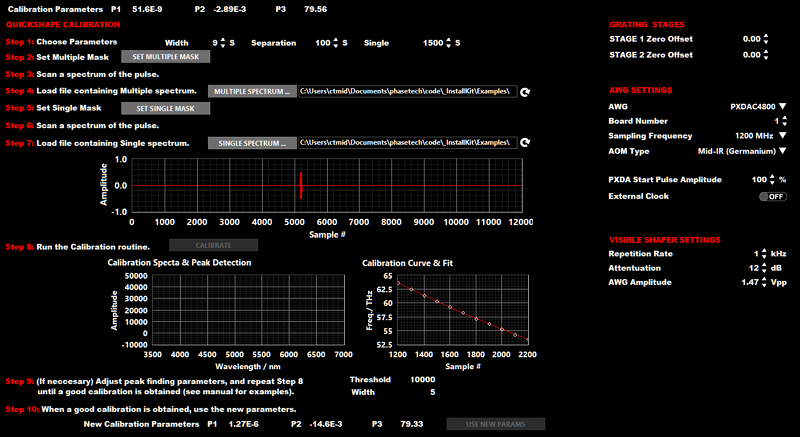
Calibration Parameters set the three parameters (P1, P2, and P3) used for spectral calibration of the shaper AOM. The parameters specify the positional distribution of spectral frequencies across the aperture of the AOM. The calibration is required for accurate calculation of shaping masks.
Following the Calibration Parameters is a step-by-step procedure for performing the calibration procedure. Calibration requires a monochromator or another method to measure the spectra of the shaper output and involves three main steps:
- Measure a spectrum of the shaped pulse with a "multiple" peak mask.
- Measure a spectrum of the shaped pulse with a “single” peak mask.
- Use the measured spectra to determine the relationship between sample and frequency and fit to a parabola.
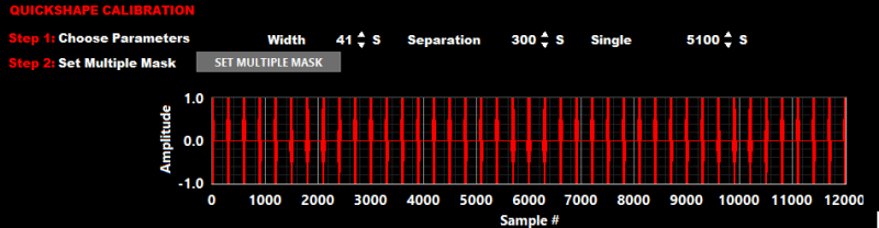
The multiple peak mask is a mask that has amplitude at discrete, regularly space positions across the RF waveform width and zero amplitude elsewhere.
The resulting output pulse has a comb-like spectrum as shown in the example below.
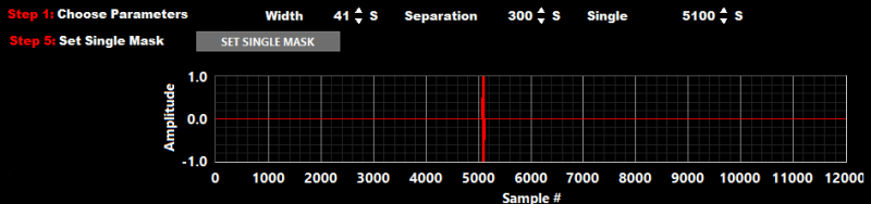
The single peak mask is a mask that has amplitude at single discrete position and zero amplitude elsewhere.
The resulting output pulse consists a single narrowband spectrum as shown in the example below.
STEP 1: Choose Parameters The first step is choose the three parameters for the masks used in the calibration procedure:
- Width: sets the width, in samples, of the peaks generated in the multiple and single masks
- Separation: sets the separation, in samples, between each peak in the multiple mask
- Single: set the center position, in samples, of the single peak in the single mask
STEP 2: Set Multiple Mask Click the Set Multiple Mask button to apply a multiple mask to the shaper using the parameters from Step 1. After applying the multiple mask it is useful to check the multiple spectrum to make sure that the parameters from Step 1 are resulting in a good multiple spectrum. The mask applied will use the amplitude value from Control Mode. In some cases, it may be necessary to temporarily increase the amplitude value to be able to observe a good spectrum.
STEP 3: Scan a spectrum of the pulse Measure a spectrum of the shaper output and save to a tab-delimited ASCII text file. This can be done with the MONO SCAN section of Acquire mode in the Advanced version of QuickControl. The file should consist of two columns with the first column consisting of wavelength in nanometers and the second column consisting of the spectral amplitude in arbitrary units.
STEP 4: Load multiple spectrum Load the file containing the multiple spectrum into QuickControl by either (1) clicking the Multiple Spectrum... button and browsing for the file or (2) entering the full file path into the text box in this step. If changes are made to the file containing the multiple file after it loaded into QuickControl, click the Refresh button to reload the file.
STEP 5: Set Single Mask Click the Set Single Mask button to apply a single mask to the shaper using the parameters from Step 1. After applying the single mask it is useful to check the single spectrum to make sure that the parameters from Step 1 are resulting in a good single spectrum. The mask applied will use the amplitude value from Control Mode. In some cases, it may be necessary to temporarily increase the amplitude value to be able to observe a good spectrum.
STEP 6: Scan a spectrum of the pulse Measure a spectrum of the shaper output and save to a tab-delimited ASCII text file. This can be done with the MONO SCAN section of Acquire mode in the Advanced version of QuickControl. The file should consist of two columns with the first column consisting of wavelength in nanometers and the second column consisting of the spectral amplitude in arbitrary units.
STEP 7: Load single spectrum Load the file containing the single spectrum into QuickControl by either (1) clicking the Single Spectrum... button and browsing for the file or (2) entering the full file path into the text box in this step. If changes are made to the file containing the single file after it loaded into QuickControl, click the Refresh button to reload the file.
STEP 8: Run the calibration routine Click the Calibrate to run the calibration routine. The routine will run a peak-finding algorithm on the multiple and single spectra and use the resulting peak positions to determine the relationship between sample number and optical frequency at the AOM.
Two graphs display the results of the calibration routine. The Calibration Spectra & Peak Detection graph will display the multiple spectrum in red and the single spectrum in white. After the calibration routine has been run it will indicate the located peak positions with squares located above each peak. The Calibration Curve & Fit curve will display a data point for each peak found in the multiple spectrum. The data points will be graphed with the sample position as the x-axis and the optical frequency, in THz, on the y axis. The data points are also fit to a quadratic equation and the fit curve is plotted on the graph as well.

STEP 9: Adjust Peak-Finding Parameters (if necessary) It may be necessary to adjust the Threshold and/or Width parameters in order to achieve a good fit. After adjusting the values, click the Calibrate button to repeat the calibration routine. To achieve a good calibration, adjust the parameters to achieve the following:
- The single spectrum has only one peak located (one white square)
- The multiple spectrum has multiple peak positions. At least three but more is better, ~8-20 is typical.
- The peaks found in the multiple spectrum are regularly spaced, no separations that are significantly larger or smaller than the others

STEP 10: Accept new parameters The calibration parameters calculated from the latest calibration attempt are displayed at the bottom of the section. Once a good fit and calibration have been achieved, click the Use New Params button to copy the new parameters to Calibration Parameters control that is used to calculate masks.

STAGE 1 Zero Offset is an offset that can be used to reset the stage position which is considered zero degrees for Grating 1. Adjust this value until the grating angle displayed in QuickControl matches the angle displayed on the physical scale on the side of the rotation stage.
STAGE 2 Zero Offset is an offset that can be used to reset the stage position which is considered zero degrees for Grating 2. Adjust this value until the grating angle displayed in QuickControl matches the angle displayed on the physical scale on the side of the rotation stage.
AWG specifies the type of arbitrary waveform generator used with the shaper. In most cases this should be set to PXDAC4800, although older shapers may use the AWG300 AWG.
Board Number is the ID number of the AWG board to use. Unless there are multiple AWG boards installed on the QuickControl computer, this number should always be one (1).
Sampling Frequency determines the rate at which the AWG will output new analog values. In most cases, this should be set to 1200 MHz. Currently the only other option is 300 MHz, however other sampling frequencies may be made available upon request. The 300 MHz sampling frequency is not compatible for use with visible wavelegth pulse shapers.
AOM Type specifies the type of crystal in the shaper AOM. Germanium is used for the mid-IR while TeO2 or quartz is used for the visible.
PXDA Start Pulse Amplitude adjusts the amplitude of the square pulse output from channel 2 of the AWG for synchronization purposes.
External Clock enables the use of an external clock signal for the sampling rate. This options is not currently available for the PXDAC4800 AWG, though it can be added upon request.
These settings are used by QuickControl to protect the AOM from permanent damage. Do not alter these settings without prior discussion and approval from PhaseTech.
Repetition Rate should be set to the repetition rate of the signal used to trigger the AWG. Typically this matches the repetition rate of the laser.
Attenuation should be set to match the attenuation factor of the inline RF attenuator placed between the AWG output and the RFA input.
AWG Amplitude this should be set to the default value of 1.47 Vpp unless otherwise instructed by PhaseTech.
This section contains a number of settings related to the collection of data from a detector as well as external channels.

Detector Type specifies the type of detector to be used with QuickControl. The "Plugin" option allows for the use of pretty much any detector via a custom-written LabVIEW plugin.
Detector Rows specifies the number of rows of pixels that the detector has.
Detector Columns specifies the number of columns of pixels that the detector has.
External Channels specifies the number of external (non-pixel) data channels that are acquired together with the detector pixel data.
Use Reference Beam enables the use of a reference beam signal to reduce the noise in the probe signal. Available for detectors with more than one row of pixels. Disabled this option if a reference beam is not available or not adequately providing good noise reduction.
The settings shown in this section will depend on the value of the Detector Type setting. Each detector has different detector-specific settings:
These settings are for PhaseTech's 2DMCT detector.
The Reinitialize button runs the initialization routine that runs at QuickControl startup.
The Setup Regions of Interest button jumps to the Control Mode Image section where regions of interest are specified.
Trigger Acquisition enables triggering of each data acquisition from the detector.
There are no detector specific settings for the MCT acquisition systems from Infrared Systems Development.
These settings are for e2v's AVIIVA line scan detector.
Integration Time sets the duration integration time window for the detector. Valid values are 1 to 6553.5 microseconds in steps of 0.1 microsecond.
Trigger Acquisition enables triggering of each data acquisition from the detector.
These settings are for some Ocean Optics Omnidriver-compatible detectors.
Integration Time sets the duration integration time window for the detector.
AWG Update Delay specifies the amount time, in milliseconds, to wait after applying a new mask to the AWG before acquiring a signal from the Ocean Optics detector. This prevent accidental acquisition of signal while the AWG is still in the update process.
These settings allow for the use of a custom LabVIEW VI plugin to acquire data from a detector.

Detector Plugin Location specifies the location of the LabVIEW VI file to be used as a the detector plugin.
The Browse button will open up a file dialog window from which the plugin VI can be selected.
These settings allow for a approximate calibration of the pixels columns of the detector. These calibrations can be used for certain graphs in QuickControl to display data as a function of frequency or wavelength instead of pixel number.
Please heed the warning displayed in QuickControl:
"Calibrations are estimates. Accuracy depends on monochromator calibration, alignment and other factors. User is responsible for verifying scientific accuracy."
Three different calibration methods are available: Basic, Advanced, and Custom. The calibration can also be disabled by choosing the None option.
Pixel column calibration is disabled.

Basic calibration uses the selected center wavelength of the monochromator, a user-supplied constant linear dispersion parameter (in units of nanometers per pixel), and the number of detector pixel columns to determine the wavelength at each pixel.

For an example, take the case of a center wavelength of 5000 nm, a dispersion of 20 nm / px, and 128 pixel columns. Since there are an even number of pixels the center wavelength is assumed to hit in between the two center pixels, 64 and 65. The wavelength at pixel 64 would then be 4990 nm and at pixel 65 the wavelength would be 5010 nm. Working in either direction with the linear dispersion of 20 nm / px, the wavelength at pixel 1 would be 3730 nm and at pixel 128 would be 6270 nm.
Advanced calibration does a more sophisticated calculation of wavelength at each pixel taking into account the geometry of the monochromator and detector, and the groove density of the monochromator grating. Like the Basic calibration method it assumes that the center wavelength of the detector is accurate
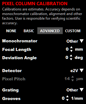
To use the Advanced calibration four parameters must be entered: (1) the focal length of the monochromator in millimeters, (2) the deviation angle of the monochromator in degrees, (3) the pixel pitch of the detector in microns, and (4) the groove density of the monochromator grating in reciprocal millimeters.
These parameters can be entered in one of two ways. First, the monochromator and detector parameters can be entered automatically by specifying the type of monochromator and detector being used with QuickControl in the Monochromator and Detector dropdown menus. The grating groove density can be also be selected using a dropdown menu - you may choose any enabled monochromator grating from the Monochromator section of the Other Devices Settings. Or you can choose the Auto option which will use the groove density of the grating selected for the monochromator in Control Mode.
Any of the parameters can also be specified manually by choosing the Other option from the dropdown menus and entering the desired parameter value.
Custom calibration allows for calibration of the wavelength at each pixel based on a set of user-specified pixel-wavelength pairs. Note that a custom calibration is only valid for a specific center wavelength of the monochromator

Use Number of Calibration Points to specify the number of pixel-wavelength pairs to use for the calibration. The values should be in the range of 2 to 5.
Underneath specify the pixel numbers and wavelengths for each pixel wavelength pair.
To determine the wavelength at each pixel column, the relationship between the pixels and the wavelengths will be fit to a polynomial of an order one less than the number of pairs specified. The fit parameters will be used to extrapolate the relationship to the other pixel columns.
These settings allow for the creation and use of a "dark" dataset from the detector which can be subtracted from subsequent detector acquisitions.
The Subtract Dark Background option enables or disables this feature. If enabled, every acquisition from the detector throughout QuickControl subtracts the dark detector data from the data acquired for each laser shot.
The Dark Background Data File specifies the location of the file containing the dark background data. The data is loaded into memory when selected or at QuickControl startup. The location can be specified by entering in the path to the file or by browsing for the location using the Browse button.
Dark Bkgnd Average specifies the number of laser shots to acquire and average when collecting new dark background data.
The Measure Dark Background button initiates the process of collected a dark background data set. When clicked, QuickControl will prompt that the detector be blocked such that no laser light illuminates the detector. Once the detector is blocked, click the OK button on the prompt. The dark background data will be acquired and a dialog box will appear in order to save the data to the desired file.
The Start Pulse Channel setting specifies the external channel to which the start pulse output of the pulse shaper is connected. If the current detection setup does not include external channel detection, this should be set to 1.has
The UV/Vis Chopper Channel settings specifies the external channel to which the sychronization signal from the opticl chopper is connected, if present.
Flip Phase will flip the phase of the pump-probe signals (positive/negative).
This section handles settings of various other devices beside the shaper and detector - monochromators and delay stages.
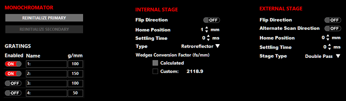
The "Reinitialize Primary" and "Reinitialize Secondary" buttons, when clicked, will run through the initialization routine for these monochromators, just as in QuickControl startup.
The Grating tables provides details about the gratings within the monochromator which are used for various purposes in QuickControl. The table has four rows to support monochromators with grating turrets that hold up to four gratings. (We don't currently know of any that hold more than three.) Each row has three inputs: a switch to enable/disable use of the grating, a string to specify a text label for the grating, and the groove density (number of grooves per millimeter) for the grating.
The gratings can be labeled however it is most useful to the user. The labels will appear in the dropdown box when selecting gratings in the Monochromator functions in Control mode. There is no effect on the function or use of the monochromator. It may be useful to specify the blaze wavelength or the wavelength range over which the grating has good diffraction efficiency.
The groove density is also displayed in the dropdown box when selecting gratings in the Monochromator functions in Control mode. Additionally, the groove density is used to provide a estimated calibration for pixel columns of the detector, if the calibration mode is set to Advanced and the Grating setting in the Advanced calibration mode is set to "Auto".
These settings pertain to the motorized delay stage within the 2DQuick IR or 2DQuick Visible spectrometers controlling the time delay between the pump and probe pulses. The settings also affect a stage being controlled through a plugin in the "Internal Delay Stage" section of Hardware Server.
The Flip Direction flips the definition of positive and negative delay relative to an absolute positive motion on the delay stage.
The Home Position is the absolute position in millimeters of the zero delay position. This setting is held in QuickControl only and does not affect any settings on the delay stage.
Settling Time specifies the number of milliseconds to wait after the delay stage has stopped moving before acquiring data.
The Type setting specifies if the delay stage is a wedge type or retroreflector type delay stage.
The Wedge Conversion Factor sets the manner through which positional movements of the traveling wedge in the wedge pair is converted to a time delay in the pulse.
These settings pertain to the motorized delay stage within the 2DQuick Transient module controlling the time delay of the actinic pulse. The settings also affect a stage being controlled through a plugin in the "External Delay Stage" section of Hardware Server.
The Flip Direction flips the definition of positive and negative delay relative to an absolute positive motion on the delay stage.
The Home Position is the absolute position in millimeters of the zero delay position. This setting is held in QuickControl only and does not affect any settings on the delay stage.
Settling Time specifies the number of milliseconds to wait after the delay stage has stopped moving before acquiring data.
If Alternate Scan Direction is enabled, experiments that scan the external delay stage over a series of delays will reverse the order of the delays for every scan. That is the scan is over delays A, B, C, ..., Z the next scan will proceed in the order Z, Y, X, ..., A. Then back to A, B, C, ..., for the following scan, and so on.
Stage Type specifies whether the external delay stage (assumed to be a retroreflector-type stage) is setup in a single-pass or double-pass configuration.
This sections contains settings and information useful for support purposes.

These options can be useful for troubleshooting issues with PhaseTech support. You may be asked to access these options under a specific set of circumstances to provide additional data to PhaseTech.
Prepare Support File will collect together a number of support files that provide information on the current state of QuickControl. It will combine these files together into a zip archive and prompt you for a location to save the zip file to. You can then send email PhaseTech the zip file when requesting support with an issue.
The Raw Data Export option will save all raw data collected by the detector and any external channels to a file. When diagnosing specific issues, PhaseTech may ask you to turn on this option, perform a specific set of steps, turn off the options again, and send back the generated data files. We do not recommend leaving this option on for extended periods of time because of the large amount of data that will be generated.
The Log File displays the contents of the log file. This file contains error messages and other details that may be useful to PhaseTech support in troubleshooting issues. The file itself is located in the main QuickControl directory and is called "log.txt".
There are two calculators built into QuickControl. The first is a calculator which calculates different parameters and performance estimates of PhaseTech pulse shapers for different wavelengths and other input parameters. The second is a calculator which calculates the frequency-domain parameters that would result from a Fourier transform of a different time-domain scan parameters.
This calculator can be used to calculate theoretical estimates for a variety of shaper parameters based on different configuration options. It can be helpful with the selection of gratings for a specific wavelenghth, changing the center wavelength of the shaper, and other uses.
all calculated values are estimates. Actual values may depend on alignment, calibration and other factors.

Shaper Type specifies the type of shaper being used, either a mid-IR or visible shaper.
Wavelength and Wavenumber specify the center wavelength or frequency of the shaper - the wavelength or frequency presumed to pass through the center of the AOM aperture for the sake of the calculations. When one is changed the other parameter is automatically updated accordingly.
Grating Grooves specifies the groove density of shaper gratings to be used for the calculations.
Mask Length specifies the length of the mask to be used for calculations in units of samples.
AWG Sampling Frequency specifies the sampling frequency of the AWG, which is rarely changed from the default value of 1200 MHz.
Grating Angle is the angle (+ and -) the gratings should be rotated to such that the center wavelength entered above will be centered on the focusing optics of the shaper.
Bragg Angle is the incidient angle into the AOM which will provide the greatest diffraction efficiency.
Spectral Window is the difference in wavelengths between the light passing through one end of the AOM aperture to the other end. The difference in wavenumbers is also shown.
Spectral Resolution is Spectral Window divided by the number of effective pixels of the AOM, which provides a limit on the maximum spectral resolution achievable with the shaper. The resolution in wavenumbers is also shown.
Max. Double Pulse Delay is calculated as 1/(twice the spectral resolution). Double pulses delays larger than this value can be generated but will suffer from a low of fidelity in pulse shape. Primarily by a decrease of amplitude of the main double pulses and the creation of extraneous satellite pulses at other time delays.
This calculator can be used to preview the frequency-domain properties that result following the Fourier transform of time-domain 2D experiments. In general, increasing the time-domain scan range increases the resulting frequency-domain spectral resolution. And decreasing the time-domain step size increases the frequency-domain spectral range. Finally, the use of a rotating frame shifts all of the resulting frequency points by the rotating frame frequency.
The calculator assumes that the time-domain data will be zero padded according to 2^ceil(log2(2*N)) points, where N is the number of time-domain steps in the scan.
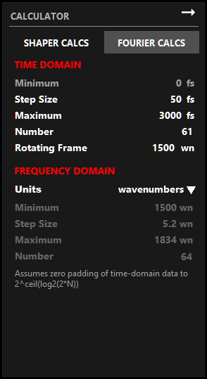
Minimum is the first time step in the time scan. This parameter cannot be modified but is displayed for clarity.
Step Size is the time between steps in the time scan.
Maximum is the last time step in the scan. It should be an integer multiple of the Step Size. Changing the Maximum value will update the Number value automatically.
Number is the number of step positions in the time scan. It equaly to the 1 + Maximum / Step Size. Changing the Number value will update the Maximum value automatically.
Rotating Frame is the frequency, in wavenumbers, of the rotating frame used in the time scane, if any.
Units provides options for the diplays units of the calculated parameters: wavenumbers, nanometers, or Terahertz. Note that the results of the Fourier transform are linear in frequency not wavelength, so when nanometers are selected as the display units the step size varies across the frequency range. Because of this a range of step sizes are displayed.
Minimum is the lowest energy frequency/wavelength after the Fourier transform.
Step Size is the step between frequency points after the Fourier transform.
Maximum is the highest energy frequency/wavelength after the Fourier transform.
Number is number of frequency points that will be produced by the Fourier transform.
The PhaseTech Hardware Server is a secondary piece of software which is required to control various hardware objects including the rotation stages in the QuickShape. If not already running when QuickControl is started the Hardware Server will be launched during QuickControl startup.
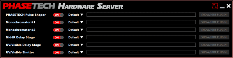
The Hardware Server allows you to enable/disable each piece of hardware can be enabled/disabled, set to use the Default hardware interface or a plugin, has a textbox for entering the plugin location as well as a button that allows the user to show or hide the plugin VI window.
To first setup the rotation stages, first turn the option for the PHASETECH Pulse Shaper to "OFF" in the Hardware Server, then enter the correct serial numbers for the two rotation stages in the QuickControl Settings screen and save all values. Then turn the option for the PHASETECH Pulse Shaper to "ON" in the Hardware Server and restart the QuickControl software.
There are seven different hardware items that can be controlled with the QuickControl hardware system.
- Detector
- PhaseTech QuickShape Pulse Shaper
- Monochromator (Primary)
- Monochromator (Secondary)
- Internal/Mid-IR Delay Stage
- External/UV/Visible Delay Stage
- Shutter
The Detector controlled through the main QuickControl software while the remaining hardware items are controlled through the Hardware Server.
All the hardware plugins use a similar structure as described below except for the detector plugin, which requires its own unique structure.
Important Notes for writing plugins:
(If using a version of QuickControl older than 0.9, plugins should be saves for LabVIEW 2012 or older.)
All plugins must have the correct controls and indicators, with the exact names, as shown below:
| error in describes error conditions that occur before this node runs. This input provides standard error in functionality. Default value is no error. Error cluster format shown below. | |
error out contains error information. This output provides standard error out functionality. Error cluster format shown below.
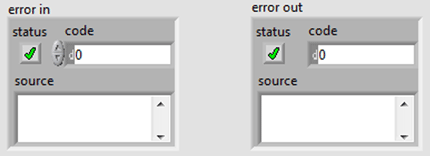
|
|
| command is a string control which will accept command strings from the QuickControl which the plugin can then parse to perform different actions | |
| wait is a boolean which must be set to false at the end of each plugin action | |
| return is a string indicator which allows the plugin to optionally pass information (for example, the current positions of a stage) back to QuickControl |
All command strings are a single line, consisting of a hardware code, an action code and an optional set of parameters, such as
MDS ABSPOS 2.3356
which instructs the plugin for the Mid-IR Delay Stage to move to a position of 2.3356 mm. Or
MONO1 GETGRATING
which requests the plugin for the Primary Monochromator to return the index of the current grating.
The plugin should be able to parse the command string into the hardware code, action code and a parameters. One possible method is using the regular expression search function:
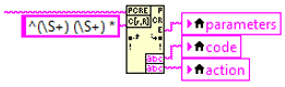
The plugin should then perform the appropriate actions for each action code based on any parameters that are passed. The recommended method for writing a plugin is through the use of event structure set to watch for a change in the value of the "command" control, parse the command string and then use a case structure to handle the different action code. A simple example is provided below.

To enable the detector plugin, go to the "DETECTION" section of Settings, and select "Plugin" for "Detector Type" in "MAIN DETECTION SETTINGS." Then enter the VI path in the "Detector Plugin Location" box.
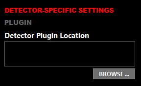
The detector plugin must have the same connector plane including the same data types (representations) as shown below.
PLUGIN DETAILS
|
error in number of shots number of pixels |
 options |
error out pixel data external channel data |
| error in test number of words is creater, and even grater to make it to one line long and then even longer still have to make the words wrap to see if ti s makes a difference and it seems like it does what hapnes if we make it to three lines. |
| error in describes error conditions that occur before this node runs. This input provides standard error in functionality. Default value is no error. Error cluster format shown below. | |||||||
| error out contains error information. This output provides standard error out functionality. Error cluster format shown below.
|
|||||||
| number of shots is the number of laser shots for which data should be acquired from the detector. | |||||||
| number of pixels is a three-element array with the number of pixel rows, number of pixel columns and number of non-detector (external) channels, in order. | |||||||
| options is a cluster with two controls - (1) "type string", a 1D array of I16 data and (2) "data string", a string control. These two controls correspond to the output of the "Variant to Flattened String" LabVIEW function. They allow for a wide variety of parameters to be passed from QC to the detector plugin. | |||||||
pixel data is a 3D array of pixel data acquired from the detector. The first array index (page) is used to separate probe and reference data:
|
|||||||
external channel data is a 2D array of external channel data acquired from the detector. The first array index (row) is used to data from the different external channels
|

The plugin option for the pulse shaper is not enabled at this time. If enabled through hardware server, the option is ignored.
Used to control the monochromator for either the probe signal or both the probe and reference signals. The plugin must handle the following commands:
| Command String: | MONO1 INIT |
| Description: | Initialize the monochromator |
| Parameters: | None |
| Return Value: | None |
| Command String: | MONO1 SETGRATING xx |
| Description: | Selects a grating, if multiple gratings are available for the monochromator |
| Parameters: | xx [I32] grating index, starting at 0 |
| Return Value: | None |
| Command String: | MONO1 GETGRATING |
| Description: | Return the index of the currently selected grating |
| Parameters: | None |
| Return Value: | [I32] grating index, starting at 1 |
| Command String: | MONO1 SETMIRROR port position |
| Description: | Sets the swing mirror positions |
| Parameters: | port [STRING] "ENTRANCE" or "EXIT" position [STRING] "SIDE" or "FRONT" |
| Return Value: | None |
| Command String: | MONO1 GETWL |
| Description: | Return the current center wavelength of the monochromator |
| Parameters: | None |
| Return Value: | [DBL] wavelength in nanometers |
| Command String: | MONO1 SETWL xx |
| Description: | Sets the center wavelength of the monochromator |
| Parameters: | xx [DBL] the desired center wavelength in nanometers |
| Return Value: | None |
| Command String: | MONO1 GETSLIT |
| Description: | Returns the current entrance slit width |
| Parameters: | None |
| Return Value: | xx [DBL] the current slit width in millimeters |
| Command String: | MONO1 SETSLIT xx |
| Description: | Sets the entrance slit width |
| Parameters: | xx [DBL] the desired slit width in millimeters |
| Return Value: | None |
To be used if the reference signal array is a separate detector than the probe signal, with its own monochromator.
Commands are identical to Monochromator (Primary), except with the hardware code MONO2
The stage used to control the delay between pump and probe pulses inside the 2D spectrometer. In older versions of QuickControl, this was called the mid-IR delay stage. In newer versions it is called the Internal delay stage.
| Command String: | MDS START |
| Description: | Initialize the stage, if necessary |
| Parameters: | None |
| Return Value: | None |
| Command String: | MDS STOP |
| Description: | Stop control of the stage, if necessary |
| Parameters: | None |
| Return Value: | None |
| Command String: | MDS GETPOS |
| Description: | Returns the current position of the stage |
| Parameters: | None |
| Return Value: | xx [DBL] the current position in millimeters |
| Command String: | MDS ABSPOS xx |
| Description: | Sets the current position of the stage |
| Parameters: | xx [DBL] the desired position in millimeters |
| Return Value: | None |
| Command String: | MDS GETSTATUS |
| Description: | Returns the current motion status of the stage |
| Parameters: | None |
| Return Value: | [STRING] either "MOVING" or "STOPPED" |
The stage used to control the delay of an additional pulse outside the 2D spectrometer, such as an actinic pulse. In older versions of QuickControl, this was called the UV/Vis delay stage. In newer versions it is called the External delay stage.
| Command String: | VDS INIT |
| Description: | Initialize the stage |
| Parameters: | None |
| Return Value: | None |
| Command String: | VDS GETPOS |
| Description: | Returns the current position of the stage |
| Parameters: | None |
| Return Value: | xx [DBL] the current position in millimeters |
| Command String: | VDS MOVEABS xx |
| Description: | Sets the current position of the stage |
| Parameters: | xx [DBL] the desired position in millimeters |
| Return Value: | None |
| Command String: | VDS GETSTATUS |
| Description: | Returns the current motion status of the stage |
| Parameters: | None |
| Return Value: | [STRING] either "MOVING" or "STOPPED" |
Can be used to block the sample from the UV/visible pump pulse in between measurements.
| Command String: | SHTR START |
| Description: | Initialize the stage, if necessary |
| Parameters: | None |
| Return Value: | None |
| Command String: | SHTR STOP |
| Description: | Stop control of the stage, if necessary |
| Parameters: | None |
| Return Value: | None |
| Command String: | SHTR SC_ENABLE |
| Description: | Set the shutter position to open |
| Parameters: | None |
| Return Value: | None |
| Command String: | SHTR SC_DISABLE |
| Description: | Set the shutter position to closed |
| Parameters: | None |
| Return Value: | None |
| Command String: | SHTR SC_GETSTATE |
| Description: | Return the current state of the shutter |
| Parameters: | None |
| Return Value: | [STRING] either "SC_OPEN" or "SC_CLOSED" |
QC now supports imaging detectors. PhaseTech's 2DMCT detector has built-in support, other imaging detectors can be used via QC's plugin system.
Added a new "IMAGE" tab to detector view in Control mode, for use with imaging detectors like the PhaseTech 2D MCT. This view is enabled when the number of detector rows is greater than 2.
- SHAPER CALCS now has an option to perform calculations for the visible AOM as well as the mid-IR AOM
- SHAPER CALCS has new input parameters for the mask length and AWG sampling frequency, so that you can see the effect of these parameters on spectral window, etc.
- SHAPER CALCS now additionally calculated the max double-pulse delay. Note this is an approximate value, there is not a sharp cutoff is usable double pulses at any particular delay.
- FOURIER CALCS can now display the calculation results in various user-selected frequency units.
A new scaling system has been created for the y-axes of the detector graph (intensity and pump-probe graph). Each y-axis now has three autoscale options: AutoScale, AutoScale Once, and Smart Autoscale:
- AutoScale: behaves like normal AutoScale function, sets the axis range to match the data each time the graph data is updated
- AutoScale Once: sets the axis range to contain the currently displayed data but does not change the range further. If AutoScale is on, selecting this option turns it off.
- Smart AutoScale: autoscale the graph once when the data exceeds the bounds of the axis range. There is a small delay to prevent autoscaling on short-lived signal changes. This option is useful for optimizing signals. For example: when making adjustments to increase pump-probe signal, turn this option on. If your changes increase the pump-probe signal beyond the axis range, the scale will update to display the full signal, but if the signal temporarily decreases a bit while optimizing, the axis range will not change on you.
All autoscale options can be also off for completely manual control over axis scales.
Additionally the pump-probe axis has an additional option to "Keep Symmetric". If on, this options will force the pump-probe axis range to be symmetric about zero. This option affects both manual and autoscale changes in the axis range.
All these axis scaling features are experimental, user feedback is appreciated.
- QC version added
- PhaseTech 2DMCT detector info added
- e2v detector info added
- Comment line in .info line is now present and comment listed as "None" if no comment is provided in QC.
- Date and time of experiment start added
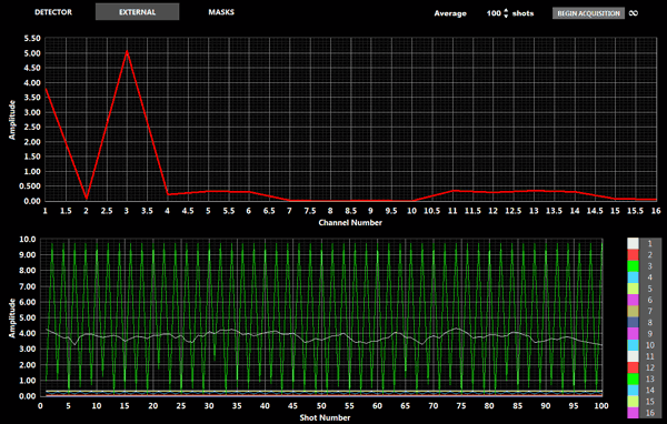
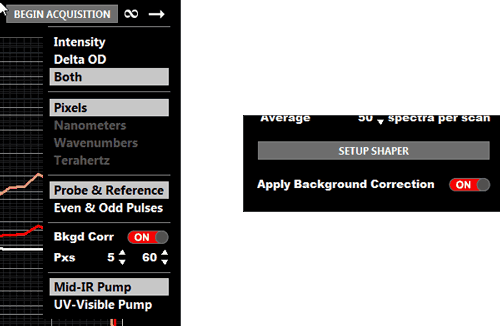 Comment - It is generally recommended to leave the background correction off for ACQUIRE mode and do the background correction in post-processing. The advantage of doing it in post is there will be more flexibility in how the background correction is done.